CelticFieldsDisplay

'Celtic Fields' – Archaeology's stepchildren
Traces of prehistoric farming in Western, Central, Eastern and Northern Europe: Displaying terrain laser data
Continue with: Interprete graphics Averaged virtual sections Generating stereo graphics Back to: Obtain terrain laser data

On three examples it is shown how I convert the laser data for an optimal illustration of the comparatively weakly pronounced 'Celtic Fields'. I work with my personal (rather outdated) program equipment, which would be hardly affordable under today's conditions: mainly Global Mapper and Surfer. The former I could buy in 2013 for 300.- €, today the (considerably extended) program can only be leased for a multiple amount per year. With Surfer I use only a function package of the much older version 6. By the way, I would like to refer to the free program packages LiVT by Ralf Hesse or RVT by Žiga Kokalj et al. which can achieve useful results for 'CelticFields' and comparable structures with suitable settings. Especially LiVT has difficulties with the calculation of larger areas (10 sqkm and more calculation area is not uncommon for Celtic Fields).

I have almost always detected 'Celtic Fields' in the shaded relief view with appropriate settings (flat azimuth, alternating illumination directions from NW to NE, appropriate superelevation settings). There are a number of problems associated: Finer linear structures can disappear in the data noise or become invisible when lying parallel to the illumination direction. Especially in terrain with high relief, such as in young glacial ground moraine landscapes or in mountainous areas, there is the problem that the illuminated slope sides are always displayed too brightly and the non-illuminated slope sides much too darkly.

Example 1: Außelbeker Gehege, Anglia, Schleswig-Holstein

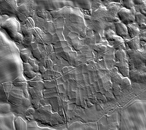
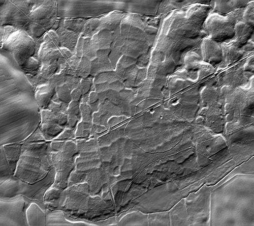
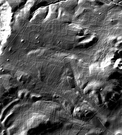
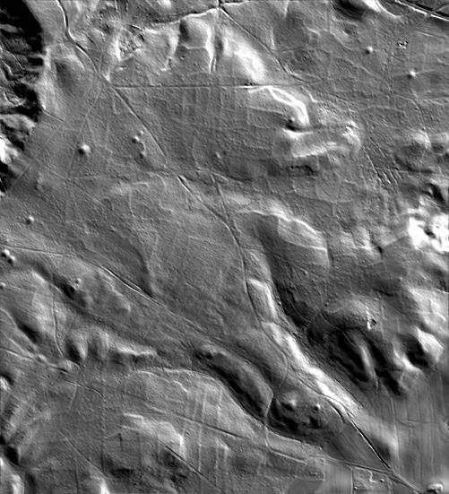
The Außelbeker Gehege as relief view (left from NW 335°, right from NE 30°). The comparison shows that linear structures lying exactly in the direction of illumination (almost) disappear. The landscape structure becomes clear in both views.

The problems with the relief views can be remedied, for example, by calculating a weighted moving average of the data matrix and subtracting this from the (possibly somewhat smoothed) original data. Basically, this so-called difference map leads to new problems: Around every small hill a kind of ring ditch is automatically created, and accordingly every round burrow gets a 'ring wall'. This is unavoidable and must always be considered when interpreting the converted data. This particularly affects very pronounced 'Celtic Fields' boundary walls or embankments, which then always appear to be accompanied by a 'ditch'. In the mountains, for example, it is also annoying that the moving mean value calculations always show hilltops a little too low and hollows a little too high. For this I have thought up a correction amount, for which a further smoothing of the moving average with the same parameters is carried out. The difference of the two mean values, multiplied by a factor, is added to the first moving mean value.

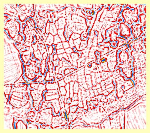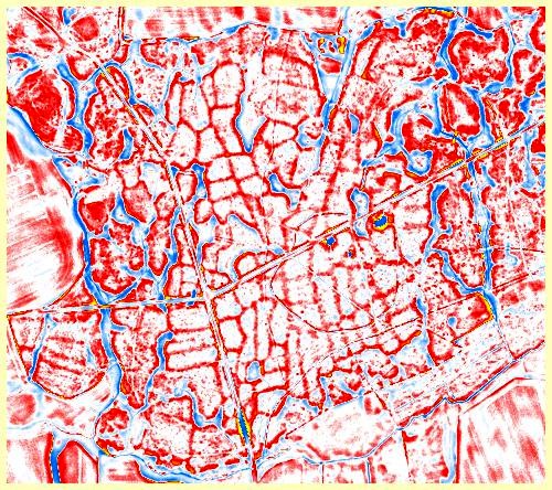
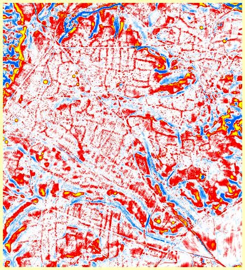
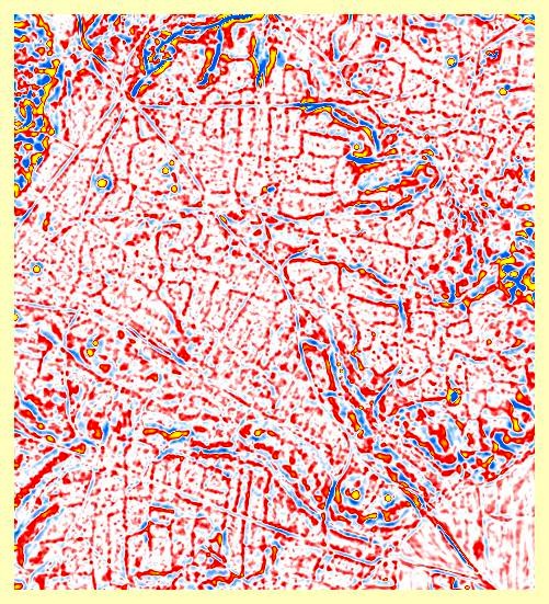
Difference maps of the Außelbeker Gehege, without hillshading only color coded, left unsmoothed without correction value, right slightly smoothed with correction value.

The two graphics clearly show the superiority of the right-hand graphic, in which a slight smoothing was first applied and then the above-mentioned correction value was included. However, the smoothing results in more or less point-like artifacts, which can be seen in the right graph especially in the east and in the northwest. Modern very narrow structures like 'Knick'-walls do not dominate anymore. The uncalculated edge of the right has become larger due to the additional smoothing calculations. By the way, the color coding (shader) is asymmetrical, much more sensitive in the positive red range than in the negative blue range. This means that slightly recessed structures such as modern forestry logging trails etc. tend to disappear. In practice, the most favorable shader is selected from a set of similar color shaders over an increasing height range.

Right: From the 30° relief image on the top left and the graphic below, this in my opinion optimal graphic was obtained by image processing, multiplying, which also still shows the structure of the landscape. Left: Smoothed difference map with correction value in relief view for information only.

Example 2: Las Marysieńka near Głubczyce, Silesia, Poland

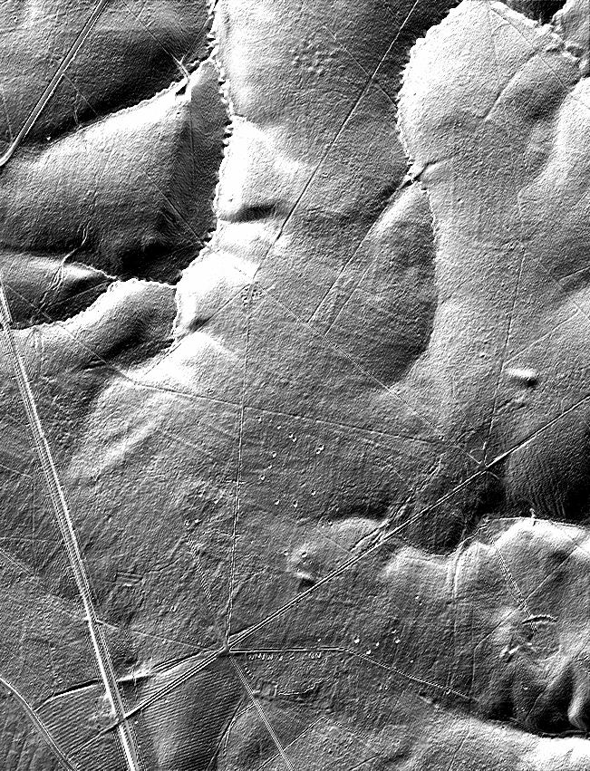
Relief graphic with two superelevation settings. On the left, the value is set a bit too high.

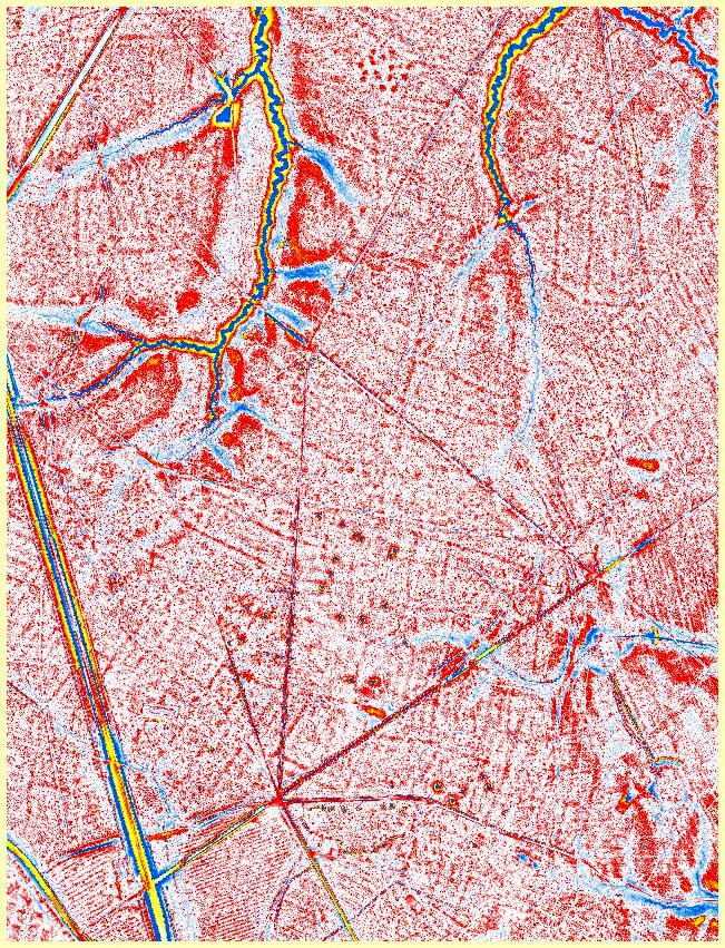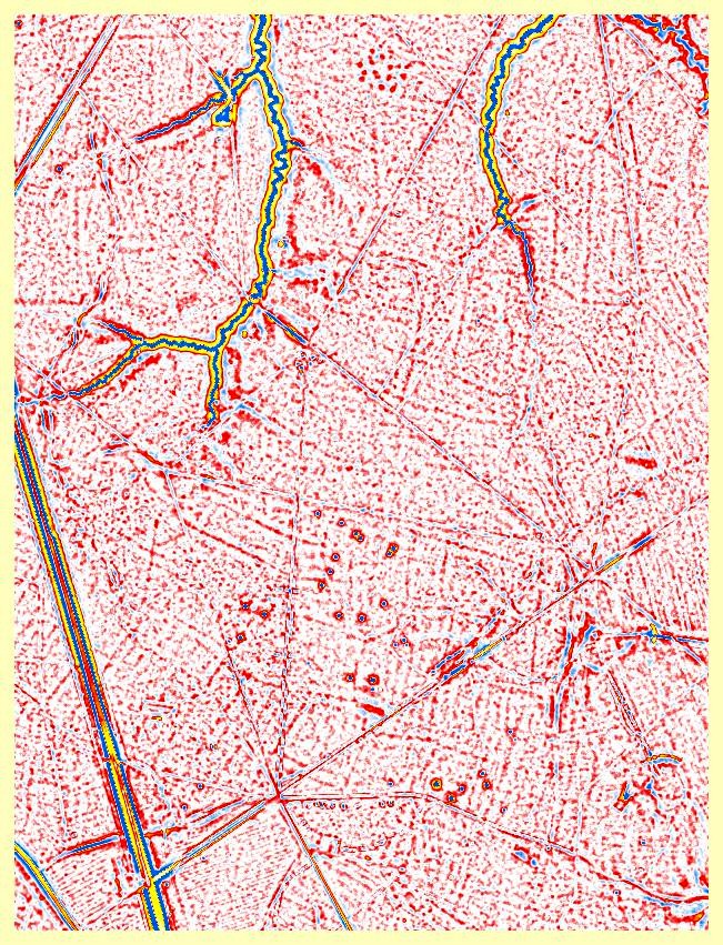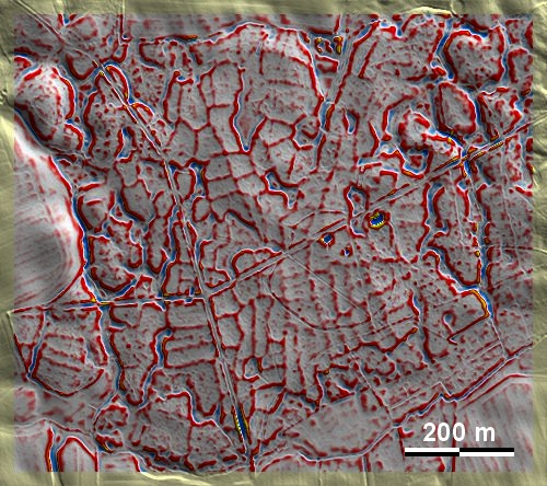
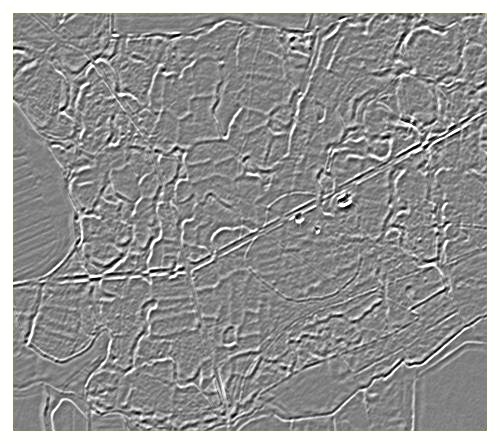
Two versions of the difference map (color coded only, without hillshading): Left unsmoothed without correction value, right slightly smoothed with correction value. On the right, the landscape structure is lost, but the weak parcel structures have become quite clear.

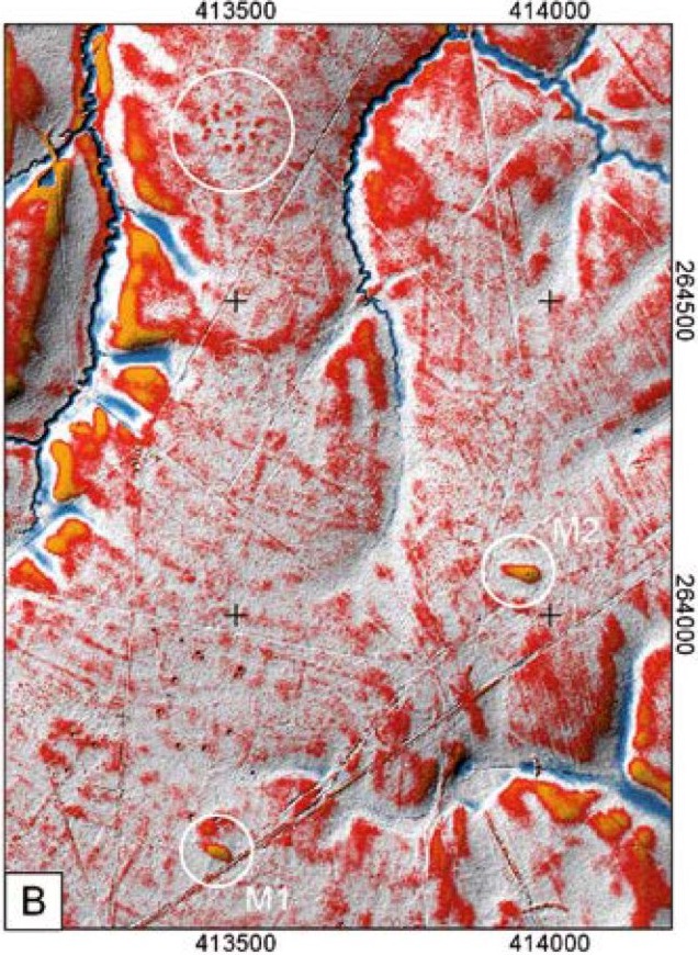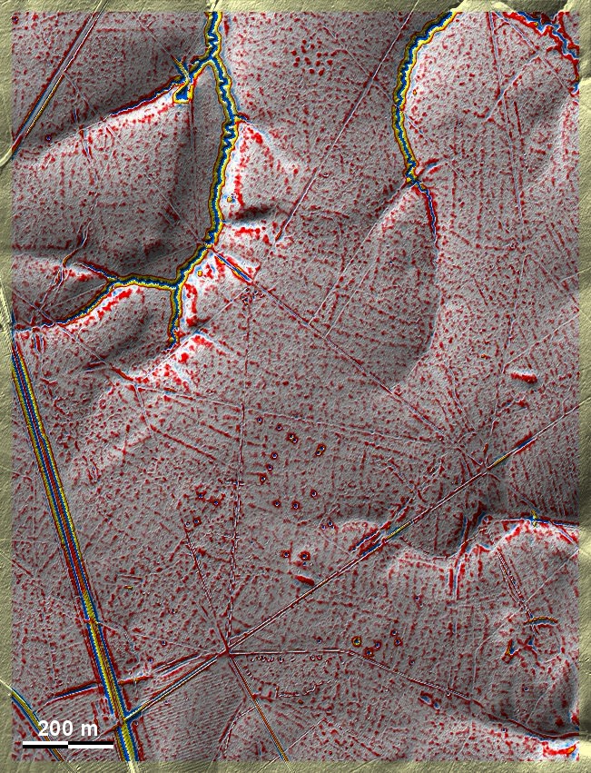
The two right graphics are combined by multiplication and in my opinion so ideal, as also shown by a comparison with a published picture (after Krupski et al.). Both the traces of former agriculture as well as the two presumably Kujawian longbarrows north of the path running from NE to SW as well as the group of small burial mounds on the middle ridge in the north become clear. The light blue shadows around the Kujawian longbarrows are, however, not real depressions but only an effect of the calculation.

Example 3: Silkeborg-Vesterskov, Jutland, Denmark

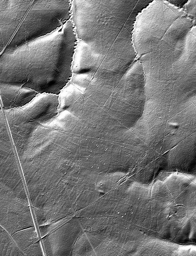
The average southeast sloping terrain is too dark in the 315° view. Better is the 45° view on the right.

Again two versions of the difference map (only color coded, without hillshading): Left unsmoothed without correction value, right slightly smoothed with correction value. On the right the landscape structure is lost, but the parcel structures have become incomparably clearer than on the left – ideal in the wildly reliefed terrain...

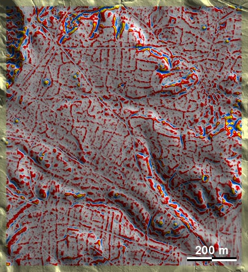
...and here is the – in my opinion – very clear combined result.

More...